Quick DFS

As we process the input from left to right, we will call each maximal sequence of equal columns a slab. For a connected column-convex region that’s a union of \(n\) rectangles there will always be at most \(2n\) slabs (they can only start and end around the ends of our rectangles), and we can find them by sweeping in \(O(n\log n)\).

The main idea of the solution is to decompose the DFS path into a reasonably small number of phases, each corresponding to a part of the run that is simple to describe. More precisely, the property we need is that within each phase we can efficiently convert between time and cell coordinates. Once we find such a decomposition, answering the queries becomes reasonably easy:

To convert time into coordinates, find the phase the time falls into and then within the phase calculate the coordinates.
To convert coordinates into time, preprocess the phases by sweeping to be able to tell, for each column, which phases it contains. Then for each query, use its column to find possible phases, among them pick the one that contains the query’s row, then convert the coordinates to the time spent within that phase, and finally add the length of all previous phases.

(Alternately, we can answer all the queries offline by sweeping both phases and queries in one pass.)

Below we present a sample run of our DFS, divided into phases in the way in which the reference solution does it.

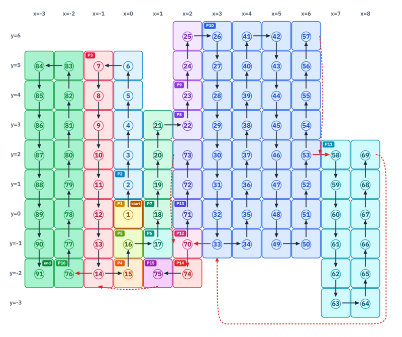
Some notes on what you see in the figure:

Cell numbers correspond to time. Black solid arrows are DFS going deeper, red solid arrows are DFS continuing after returning from an explored branch.
Red dashed arrows represent moments when the reference solution makes a resume jump. These are the moments when we have fully explored some region and now we need to go back down the original DFS stack until we get to the first cell from which we can continue exploring. (This may require repeated popping from our own stack to return to the correct previous phase.)
Phases are color-coded and numbered starting from P1.
Each phase is a single step, a single walk in one direction (which is either N or S), or a sweep of a 2D area (explained below).
Single steps are self-explanatory, and we use them whenever nothing else fits.
A walk northward can be performed whenever the cell in the N direction is unexplored. (While that is true, take a step north.) Similarly, a walk southward is available whenever the cell to the north is already visited and the one to the south is available. Examples of these are P2, P5, P7, P9, and P3, P14 for the other direction.
The most complex type of a phase is a serpentine sweep, as shown in P10 and P11 eastwards and P16 westwards. In P10, upon entering a clean column on the top eastwards, we know that the DFS is going to sweep the whole rest of the slab before anything else happens. Instead of simulating it one step at a time, we can just call it a phase and move on. This is the main way of filling a lot of space quickly.

When going westward we need to be a bit more careful because going east takes precedence. Observe how P3 does not start a sweep westwards yet, as from its bottom (cell 14) we first have to continue to the east. (In code, P3 may be implemented as a sweep that gets interrupted early instead of a walk. It does not really change anything.)
In order to be able to quickly determine where to continue once we hit a dead end, we’ll need to keep track of the frontier of the already explored area: the blocks of already explored cells that still have unexplored neighbors. For example, observe the situation after exploring cell 57. At this moment in time we need to be able to tell that the correct next cell to which we need to backtrack is cell 53: the most recently visited cell that still has an unexplored neighbor.

More details on sweeps

We will only start a sweep eastwards under the following conditions:

The current cell has both N and S direction unavailable, and the E direction is available.
The cell in the E direction is either the lowest or the highest in its column.
That column has not been visited yet.

For a sweep westwards we need to add one additional check:

Once we take the step left and fill the first empty column, if we went southwards, we need to check whether the last cell still has an unvisited neighbor to the east. If it does, this phase will be just a walk southwards instead of a sweep.

(We may do the same check when walking northwards if it leads to a simpler implementation, but it’s never necessary. Let \(C\) be the cell from which we entered the first empty column. As we just went from \(C\) westwards, we can deduce that everything northwards of \(C\) has already been visited – for every cell \(X\) that was previously visited, its northern neighbor, if any, must have also been previously visited, at the latest immediately after \(X\). Thus, if we go from \(C\) west and then northwards, there surely won’t be any unvisited cell to the east of that column. Phase P3 in the above figure shows that we do need the check at least when going southwards.)

A multicolumn sweep always continues all the way to the end of the slab. (The visited columns are always one contiguous block, so when we start sweeping by going to an empty column, the rest of the slab in that direction must be empty too.)

Where to resume?

At any moment \(t\) of our simulation of the DFS, we can look at the entire set \(V_t\) of the first \(t\) visited cells, and we can define its frontier: the cells of \(V_t\) that have at least one neighbor in \(R \setminus V_t\). Whenever our current branch of DFS terminates, the DFS is going to repeatedly pop from its stack until it returns to the most recently visited frontier cell.

Instead of keeping track of the individual frontier cells (there can be way too many of them) our stack will contain the phases created so far – more precisely, only those of them that still may have some frontier. Whenever we discover that the topmost phase on the stack no longer has any frontier, it can be popped. (Once a phase has no frontier, it will never regain any.)

Then, the next resume cell will always be the maximum-time frontier cell of the topmost phase in the stack.

What does the frontier of a phase look like?

If we have a multicolumn sweep (i.e., with more than two columns), the middle columns obviously cannot contain frontier cells. So for sweeps it’s enough to look at their leftmost and rightmost column. Both other phase types are entirely within one column.

Within any single column of any type of phase, visit time is strictly monotone (grows north-to-south or vice versa).

Thus, for any such column we can find the maximum-time frontier cell it contains in constant time, as follows:

Let \([lo,hi]\) be the range of \(y\)-coordinates covered by the phase, and let \(x\) be the column we are examining.
Within each of the columns \(x\pm 1\), we need to check for the extreme unvisited cells (highest or lowest; we can always just check both) within the range \([lo,hi]\).
Within column \(x\) itself we need to check cells with \(y\)-coordinates \(lo-1\) and \(hi+1\).

Each of these neighboring cells, if they exist and are unvisited, has precisely one already visited neighbor in the examined column \(x\). That neighbor is now a candidate for the maximum-time frontier cell within the examined column. The most recently visited among those candidates is then the answer we seek.

Keeping track of unvisited cells

As we are always going north first, we can make the following observation (which is then easily proved by induction): Outside of the currently active run northwards (if any), the visited cells in any partially-visited column \(x\) form a single interval \([v(x), hi(x)]\). In other words, the unvisited cells form a single “pocket” \([lo(x), v(x)-1]\) at the southern end of the column.

Each of these pockets has to be re-entered later. This can only happen in two ways: either from the top, or from an adjacent column.

In order to efficiently access information about unvisited cells, we will store it as follows:

An ordered set of maximal intervals of columns in which all cells are visited.
Separately for each partially-visited column its current state. (The state is either just one visited cell, just one visited interval from somewhere to the north edge, or that interval + one isolated cell below where we just re-entered the column. If the state involves an isolated cell, the very next phase will go northwards and fill in the gap above it.)

With these data structures we can perform all necessary operations (checking whether a column was already visited, finding extremal unvisited cells, etc.) in logarithmic time.

The number of partially-visited columns

In the previous section we may have grown concerned whether e.g. the data structure for all partially-visited columns won’t be too big. We will now see that it won’t be. More precisely, the total number of partially-visited columns will always be linear in \(n\).

An unvisited column that is first entered at one of its endpoints is immediately traversed completely. Therefore, partially-visited columns can only arise from the starting cell (there’s obviously exactly one of these) and then from situations where we enter a clean column from its neighbor, and somehow that step sideways will bring us into one of the new column’s interior rows.

(Observe that the phase that creates a new partially-visited column always consists of a single step.)

Sometimes that step may be taken across the boundary between two slabs. There are fewer than \(2n\) such boundaries and thus fewer than \(2n\) moments when a new partially-visited column appears this way.

Now suppose that a clean column \(c\) is first entered at an interior cell from a neighboring column \(d\) that is in the same slab. We will show that this can only happen once in the whole region: for \(c=-1\) and \(d=0\).

As \(c\) and \(d\) span the same rows, any attempt to step from \(d\) towards \(c\) succeeds while \(c\) is clean. Hence, the step that enters \(c\) must be the very first attempt made from any cell of \(d\) in the direction of \(c\). Where and how can this happen?

First, note that if \(d\) was first entered at one of its endpoints, the DFS will traverse all of \(d\) and the first cell of \(d\) from which we’ll eventually try to enter \(c\) will be the cell at the opposite endpoint of \(d\). But as \(c\) and \(d\) are in the same slab, this would mean that we enter \(c\) at its endpoint.

Second, it’s not much different if \(d\) was first entered in the middle, which must have been from some cell \(E\) in its other neighbor \(e\). Once the DFS enters \(d\), it will walk all the way to the top of \(d\). Let that topmost cell in \(d\) be \(D\). What happens next? As we already moved from \(E\) sideways, this means that all cells above \(E\) in \(e\) are already visited. Thus, there cannot be an available unvisited cell to the right of \(D\). But this means that the DFS will continue into the topmost cell of \(c\). Again, we entered \(c\) at its endpoint, not in the interior.

This leaves us with only one other option: \(d\) cannot have been entered at all, which means that it’s indeed the starting column (and the starting cell is in its interior).

The above already concluded the proof, but for completeness we’ll also show that the situation we’re analyzing can actually happen in this specific scenario. It will look as follows: the DFS starts from the starting cell in column \(0\) northwards, then it continues eastwards, and eventually it returns from there to re-enter column \(0\) in an unvisited cell below the starting one. From there the DFS would then enter column \(-1\) in one of its interior cells.

This proves that the total number of partially-visited columns during the entire run of our algorithm is linear in \(n\).

The number of phases

Once we create a partially-visited column, some careful casework can show that during the entire run of the rest of the DFS this column can only be reentered at most twice. More precisely, we can show that the column can only be reentered at most once from each side. This type of reentry must happen at one of two locations: either immediately below the lowest previously visited \(y\), or at the lowest \(y\) coordinate the pair of columns has in common. Additionally, there is one more way in which we can get exactly one new phase within a column that is currently partially visited: the DFS returns to the southmost visited cell in the column and continues southwards from there to fill the rest of the column. This means that each column that starts as partially-visited will eventually be fully covered by a small constant number of phases.

We also know the only condition that can prevent a sweep within a slab – see end of phase P3 in the example at the beginning. And as that condition can only happen at most once per slab, we know that the total number of multicolumn sweep phases is at most linear in \(n\) (at most one such sweep per slab) and that within each slab at most a constant number of columns isn’t covered by a sweep.

Together, these observations show that the total number of phases is linear in \(n\). Thus, the entire DFS simulation runs in \(O(n \log n)\) time and \(O(n)\) space. We already explained above how to answer the queries in \(O(q\log (n+q))\).